Forecasting CO2 allowance prices in the European ETS market
A two-stage econometric approach
Published by Martina Gallus. .
Energy Analysis tools and methodologiesThe European ETS market
The European ETS market is a cap-and-trade system in which a maximum cap is set on total emissions. Companies subject to the system must hold enough allowances to cover their emissions, while financial operators can trade allowances as market assets.
The price of CO2 allowances therefore reflects a complex set of factors: financial expectations, European climate policies, energy prices and the composition of electricity generation. This dual nature, regulatory and financial, makes the price of ETS allowances particularly difficult to forecast in the short term.
Model objectives
The objective is to build an econometric model capable of forecasting the expected average price of CO2 over a horizon of the following 15 days. The forecast is not based on a simple extrapolation of the current price, but combines information from the futures curve with variables linked to energy fundamentals, in order to capture both financial expectations and energy market conditions.
The CO2 forecast represents an important component for the subsequent construction of an hourly PUN forecasting model. The price of ETS allowances affects the generation costs of fossil fuel plants and will therefore be used, in subsequent models, as a baseline variable to explain and forecast the dynamics of wholesale electricity prices in Italy[1].
Data
The final dataset has daily frequency and combines PricePedia financial data with ENTSO-E data, originally available at hourly frequency and subsequently aggregated at daily level. In the final model, the first stage uses 766 observations, while the second stage is estimated on 765 observations.
The following table describes the main variables used in the two stages of the model.
Variables used in the CO2 model
| Variable | Source | Frequency | Description |
|---|---|---|---|
| CO2, C6M, C12M | PricePedia | daily | Continuous futures with maturities at 1, 6 and 12 months. |
| TTF1, TTF6, TTF12 | PricePedia | daily | Continuous TTF futures with maturities at 1, 6 and 12 months. |
| Fossili | ENTSO-E | hourly → daily | Electricity generation from fossil sources, aggregated by day. |
| FOSS_Carbone | ENTSO-E | hourly → daily | Electricity generation from coal, aggregated by day. |
Model structure
The model is structured in two stages. The first stage estimates the expected average price of CO2 over the following 15 market days, indicated as CO2_15. The second stage instead describes the daily variation in the CO2 price, considering both the movement of the target estimated in the first stage and the correction of the deviation from that target.
First stage - variables and interpretation
CO2_15 = 11.5583 + 0.8643CO2 + 0.8459DIFF_C12M + 0.0133CARB_GAS
| Regressor | Coeff. | Std. err. | t | p-value |
|---|---|---|---|---|
| const | 11.5583 | 1.069 | 10.811 | 0.000 |
| CO2 | 0.8643 | 0.014 | 60.141 | 0.000 |
| DIFF_C12M | 0.8459 | 0.178 | 4.761 | 0.000 |
| CARB_GAS | 0.0133 | 0.003 | 5.288 | 0.000 |
|
0.865
R2
|
766
Observations
|
0.195
Durbin-Watson
|
0.864
Adjusted R2
|
The following variables were implemented for the estimation of the first-stage model:
The dependent variable, as indicated, is CO2_15. This variable represents the future moving average of the CO₂ price over the following 15 days. The choice of using CO2_15, instead of the simple current price of the 1-month CO₂ future, responds to the need to orient the model toward forecasting.
Regressors:
- CO2 (coeff. 0.8643): 1-month CO₂ future. The positive coefficient (see the table reported below) is close to 1. It indicates that this variable captures the strong persistence of financial prices. A change of +1 €/t recorded today determines a change of +0.86 €/t in the expected average price over 15 days.
- DIFF_C12M (given by the difference CO2 – C12M, coeff. 0.8459): It measures the distance between the 1-month EUA future and the 12-month EUA future. This variable is positive when the expected price at one month is higher than the expected price at 12 months. This means that the market expects greater demand pressure at one month than in the medium term. The positive coefficient of this regressor therefore tends to capture the greater pressure concentrated on the short end of the curve.
-
CARB_GAS (coeff. 0.0133): This variable captures the effect due to the mix of energy sources used, known in the literature as the fuel switching phenomenon, that is, the substitution between different energy sources in electricity generation. When the gas price, or the expectation of the future gas price, increases relative to other fossil sources, operators have an incentive to reduce gas use and increase reliance on coal. This causes an increase in CO2 emissions and, consequently, upward pressure on the CO₂ price. The variable used in the regression is given by the product of these two components:
- As the first component, the share of electricity generation from coal over total fossil energy sources was used, and then a 30-day moving average was calculated: SH_CARB_MM30.
- To assess its joint effect on the future price of CO2 allowances, the share of energy produced from coal was multiplied by the difference between the 12-month and 1-month TTF futures: ( TTF12 - TTF1), which captures expectations on the gas price.
The positive and significant coefficient confirms that the variable, as constructed, captures a non-linear effect: the effect of the share of coal used in the energy mix is not constant, but also depends on expectations on the gas price.
CARB_GAS = SH_CARB_MM30 × (TTF12 − TTF1)
When coal use increases and gas is expected to become more expensive, the effect on the demand for allowances is amplified. It is worth noting that the model was also tested using only the variable SH_CARB_MM30, without interaction with the gas curve. Also in that specification, the coefficient of the coal share is positive and statistically significant. This confirms that the weight of coal in fossil generation is itself a relevant driver of the CO₂ price. The introduction of CARB_GAS therefore represents a deliberately introduced complication, not because the coal share alone does not work, but to better understand the joint dynamics between expectations on the gas price and coal use.
The model explains about 86.4% of the variability of the expected average price over the following 15 days. All regressors are statistically significant.
Second stage – variables and interpretation
Δ CO2t = 1.1355 ΔCO2_15EQt - 0.0189 ERRt-1
The second stage estimates the short-term dynamics, that is, the daily dynamics of the price of the 1-month CO2 future. While the first stage estimates an expected value at 15 days, the second stage analyzes how the current price moves relative to that estimated value. Using equation 1), the fit of the equation was calculated, which can be considered the equilibrium value toward which the actual price of CO2 certificates progressively adjusts.
| Regressor | Coeff. | Std. err. | t | p-value |
|---|---|---|---|---|
| DCO2_15EQ_t | 1.1355 | 0.008 | 148.723 | 0.000 |
| ERR_R1 | -0.0189 | 0.008 | -2.381 | 0.017 |
|
765
Observations
|
0.967
R2 uncentered
|
2.396
Durbin-Watson
|
1.9%
Correction speed
|
Dependent variable:
ΔCO2t : CO2t – CO2t-1 measures the daily variation in the price of the 1-month CO2 future.
where Δ represents the first difference
Regressors:
- ΔCO2_15EQt ( CO2_15EQt - CO2_15EQt -1, coeff. 1.1355 ): Variation in the fit estimated in the first stage. It measures how the expected value of CO2 at 15 days estimated by the first stage changes from one day to the next. The coefficient is positive and significant: an increase of 1 €/t in the estimated CO2_15EQ value is associated with an increase of about 1.14 €/t in the daily variation of CO2. The current price follows the movement of the estimated equilibrium value almost entirely, in a more than proportional way
- ERRt-1 (CO2t-1 - CO2_15EQt-1, coeff. -0.0189 ): This variable represents the ECM term, that is, the error correction term. It serves to verify whether there is a mechanism of return toward the equilibrium value calculated in the first stage. The coefficient is significant and negative, as it should be, based on how it was constructed. This result indicates that, when CO2 is above the estimated equilibrium value, it subsequently tends to decrease; when it is below, it tends to recover. The correction speed is equal to a daily recovery of 1.9%

Conclusions
The results obtained show that futures curves add relevant information to explain the short-term dynamics of ETS allowance prices. In particular, the slope of the EUA curve helps to understand whether price pressures are concentrated in the short term or distributed over a longer horizon.
An interesting result also concerns the indirect effect of the share of coal in the energy mix. The interaction between the share of coal in fossil generation and the slope of the TTF curve makes it possible to capture the fuel switching mechanism: greater use of coal, combined with expectations of more expensive gas, can translate into higher expected emissions and therefore upward pressure on CO2 prices.
Overall, the model represents a good starting point to reduce the complexity of ETS price forecasting, combining financial information and energy fundamentals.
Finally, the second stage shows that daily CO2 variations are mainly explained by the movement of the equilibrium value estimated in the first stage. The ECM term confirms the existence of a mechanism of return toward equilibrium, but the adjustment is slow. The negative and significant coefficient of the error term indicates that, when the price deviates from the estimated short-term value, it subsequently tends to correct part of the imbalance.
Do you want to stay up-to-date on commodity market trends?
Sign up for PricePedia newsletter: it's free!
[1] For a description of the model of the single national price (PUN) for electricity in Italy: https://www.pricepedia.it/it/magazine/article/2026/05/25/come-si-forma-il-pun-orario-il-ruolo-della-domanda-residuale-e-della-dinamica-intraday/
[2] Electricity generation data by source: ENTSO-E Transparency Platform
You may be interested in:
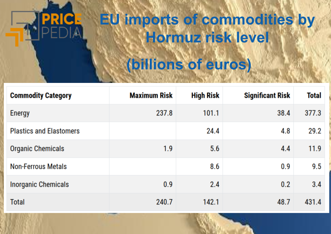
Supply Risk in the Event of a Closure of the Strait of Hormuz
Published by Luigi Bidoia. .
Energy Organic Chemicals Petrolchimica Strait of HormuzLe commodity europee maggiormente esposte al rischio Hormuz [ Read all ]

The effect of renewables on the Italian hourly electricity price
Published by Emanuele Morelli. .
Energy Electricity's National Single Price Electric Power Machine learning and EconometricsUn'analisi econometrica sul periodo gennaio 2023 - giugno 2025 [ Read all ]
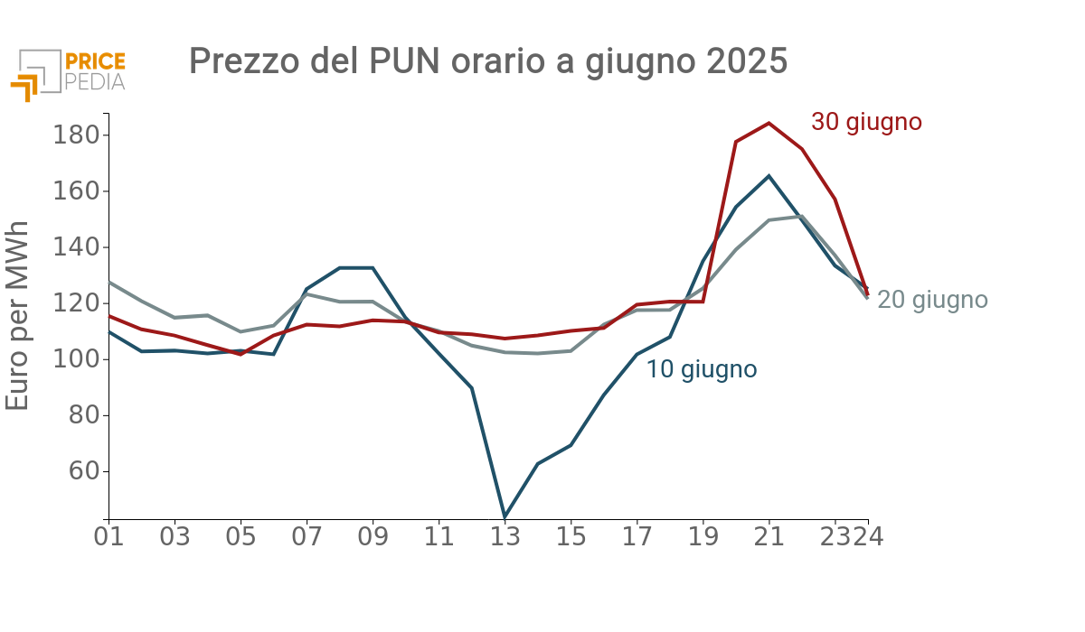
How renewable energy is changing hourly electricity prices in Italy
Published by Emanuele Morelli. .
Energy Electricity's National Single Price Electric Power Machine learning and EconometricsIn June, the hourly structure of the Italian electricity price (PUN) changed radically, as clearly shown in the graph below. This change fits into a longer-term trend. In recent ye}... [ Read all ]