How the Hourly PUN Is Formed: The Role of Residual Demand and Intraday Dynamics
An econometric model shows how renewables, residual demand, and hourly profiles influence electricity prices in Italy
Published by Martina Gallus. .
Electricity's National Single Price Price DriversIntroduction
In the article
How much renewables reduce the dependence of the PUN on gas prices
,
a model was presented that explains a large part of the dynamics of the hourly PUN over the last two years.
The analysis showed that gas prices are still the main determinant of electricity prices, but also that the growing share of generation from renewable sources helps reduce this dependence.
In this follow-up analysis, the model was extended with the aim of identifying additional factors able to improve its explanatory power for hourly variations in the PUN.
The analysis highlighted two particularly relevant elements:
- residual demand with respect of the demand satisfied by renewable sources;
- the intraday structure of the price.
Residual demand as a determinant of the PUN
A first improvement of the model consists in introducing the residual demand, that is the share of electricity demand that remains to be met after the contribution of generation from renewable sources.
This residual demand is calculated as:
DOM_RES = DOM × (1 − SFER)
where SFER represents the share of electricity generation produced from renewable sources.
The following table compares the estimated coefficients with and without the introduction of this variable:
Estimated coefficients of the hourly PUN equation
| Variable | Without residual demand | With residual demand |
|---|---|---|
| Constant | -25.1314 | -58.2963 |
| Standard variable cost (euro/MWh) | 1.0244 | 1.0208 |
| Electricity demand (GWh) | 1.9734 | 0.6138 |
| Residual electricity demand (GWh) | 2.3309 | |
| Share of electricity generation from renewable sources | ||
| below 70% | -0.3244 | 0.4637 |
| between 70% and 80% | -0.6020 | 0.1846 |
| above 80% | -0.9398 | -0.1506 |
| Solar share in renewables (%) | -0.5056 | -0.4771 |
| Wind share in renewables (%) | -0.2652 | -0.2426 |
| Dummy variables | ||
| non-working days | 9.5776 | 8.8065 |
| winter days | -1.2809 | -2.2106 |
| summer days | -1.8059 | -1.3022 |
Regression statistics
| Statistic | Without residual demand | With residual demand |
|---|---|---|
| R2 | 0.757 | 0.765 |
| Durbin-Watson | 0.400 | 0.412 |
- R2 and overall fit: introducing the residual demand among the model regressors increases the R2 statistic from 0.757 to 0.765, suggesting that this variable improves the model’s ability to account for variations in the hourly PUN.
- Role of gas: even after introducing the variable related to the residual demand, the coefficient associated with the marginal cost of gas remains close to one, indicating an almost complete pass-through between the marginal cost of gas and the electricity price.
- Demand coefficient: with the addition of the residual demand variable, the coefficient of demand drops sharply, while the coefficient of residual demand becomes dominant. The estimated coefficients clearly show that the market reacts more strongly not to total demand, but to the share of demand that must be met by conventional generation after the contribution of renewables.
-
Effect of renewables: in the model without the residual demand variable, as described in the article mentioned above, electricity generation from renewable sources has a negative effect on the PUN price, an effect that increases as their share grows. This result is consistent with the Merit Order Effect.
In the model including residual demand, however, some coefficients related to the share of electricity generation from renewable sources even become positive. Much of the effect of renewables on prices operates indirectly through the reduction in residual demand. The SFER dummy variables therefore become "residual" variables with respect to the effects captured by the residual demand variable. - Photovoltaics and wind power: the photovoltaic and wind shares have negative coefficients, as expected, in both models, with a higher coefficient in absolute value for photovoltaics.
Intraday dynamics and harmonic functions
Even after including residual demand in the model, the model errors show strong positive autocorrelation, as highlighted by the rather low Durbin-Watson statistic (0.412). As shown by the chart representing the average error across the different hours, there is a certain systematic pattern in the structure of the errors.
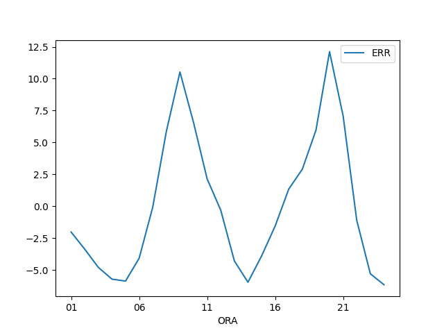
The model errors show a clear systematic structure over the course of the day. In particular, the model tends to overestimate and underestimate the PUN always in the same hours. After the negative error values recorded during the night hours, the error shows a first phase of growth in the morning hours, with a peak around 9-10. This is followed by a reduction during the central hours of the day and a second growth phase, with a higher peak in the evening hours.
This evidence suggests that electricity prices have a systematic component linked to the hour of the day that is not explained by the fundamental variables. The shape of the errors suggests the possible existence of harmonic components. In order to test this hypothesis, we considered two different harmonic functions[1]:
- one with a 24-hour periodicity, associated with the day-night alternation;
- one with a 12-hour periodicity, characterized by two maxima and two minima over the course of the day.
The first estimation results confirmed the validity of this hypothesis. They also suggested that this intraday structure is strongly associated with the profile of photovoltaic generation. To test this second hypothesis as well, we introduced new variables given by the product between the harmonic components and the share of photovoltaic generation. The results for these additional variables were also statistically significant. This indicates that the contribution of the harmonics becomes more relevant precisely during the hours when photovoltaic generation is higher.
Estimated coefficients of the hourly PUN equation
| Variable | Without residual demand | With residual demand | With residual demand + harmonics |
|---|---|---|---|
| Constant | -25.1314 | -58.2963 | -4.1125 |
| Standard variable cost (euro/MWh) | 1.0244 | 1.0208 | 1.0070 |
| Electricity demand (GWh) | 1.9734 | 0.6138 | 0.6522 |
| Residual electricity demand (GWh) | 2.3309 | 0.8538 | |
| Share of electricity generation from renewable sources | |||
| below 70% | -0.3244 | 0.4637 | -0.1388 |
| between 70% and 80% | -0.6020 | 0.1846 | -0.4043 |
| above 80%% | -0.9398 | -0.1506 | -0.7192 |
| Solar share in renewables (%) | -0.5056 | -0.4771 | -0.4333 |
| Wind share in renewables (%) | -0.2652 | -0.2426 | -0.1707 |
| Dummy variables | |||
| non-working days | 9.5776 | 8.8065 | 3.7068 |
| winter days | -1.2809 | -2.2106 | -2.4957 |
| summer days | -1.8059 | -1.3022 | 0.7412 |
| First harmonic | |||
| cosine component | -6.4045 | ||
| sine component | -7.8966 | ||
| Second harmonic | |||
| cosine component | -0.3449 | ||
| sine component | -7.0121 | ||
| First harmonic times photovoltaic share | |||
| cosine component | -0.1393 | ||
| sine component | 0.3446 | ||
| Second harmonic times photovoltaic share | |||
| cosine component | -0.1588 | ||
| sine component | 0.0488 | ||
Regression statistics
| Statistic | Without residual demand | With residual demand | With residual demand + harmonics |
|---|---|---|---|
| R2 | 0.757 | 0.765 | 0.803 |
| Durbin-Watson | 0.400 | 0.412 | 0.479 |
The estimation results show a significant improvement in both R2 and the model’s predictive accuracy. They also provide the following insights into the harmonic structure of the intraday price:
- First harmonic: the first harmonic captures the day-night structure of the electricity market. All coefficients are significant, highlighting a strong systematic oscillation of the PUN over the 24-hour period.
- Second harmonic: the second harmonic represents a semi-daily periodicity. Economically, this is consistent with the fact that the electricity market does not have a single daily peak, but rather an articulated intraday structure, characterized by lower prices during the night hours, an increase in the morning hours, compression during the central hours, and a new rise in the evening hours.
-
Effect of photovoltaics on the intraday structure: the interactions between harmonics and the photovoltaic share are largely significant. The results suggest that photovoltaics affect not only the average level of the PUN, but also its intraday structure, influencing:
- the amplitude of oscillations;
- the timing of price peaks.
The temporal dynamics of errors and the ECM model
Despite the improvement obtained with the inclusion of residual demand and the harmonic components, the model errors continue to show autocorrelation, as indicated by the low Durbin-Watson values.
This suggests that the price formation process is not fully instantaneous: the observed PUN tends to deviate from its equilibrium value, and this deviation persists over time before being gradually absorbed.
To capture this dynamic, an ECM (Error Correction Model) was estimated according to the Engle and Granger approach, structured in two stages. The cointegration analysis confirms the existence of a long-run equilibrium relationship between the PUN and the main explanatory variables considered in the model.
In the first stage, the long-run relationship between the PUN and its fundamentals is estimated, namely the static model already described above, whose residuals measure, hour by hour, how much the observed price deviates from equilibrium.
In the second stage, a short-run equation is estimated in which the hourly variation of the PUN depends on the variation in the equilibrium price and on the disequilibrium accumulated in the previous hour: if the PUN was too high, it tends to decrease; if it was too low, it tends to increase.
The functional form of the short-run equation and the estimation results obtained are reported below.
ΔPUNt = α + βΔ PUN t + λECt-1 + εt
where:
-
Δ is the first-difference operator, therefore:
- ΔPUNt = PUNt − PUNt-1
- Δ PUN t = PUN t − PUN t-1
- PUN t represents the fit of the long-run equation;
- ECt-1 represents the error of the long-run equation in the previous hour.
Estimated coefficients of the ECM model
| Variable | Coefficient | t-stat |
|---|---|---|
| Constant | -0.0009 | -0.016 |
| Δ PUNeq | 0.9497 | 151.395 |
| ECt-1 | -0.2384 | -62.008 |
Summary indicators
| Statistic | Value |
|---|---|
| R2 | 0.480 |
| Durbin-Watson | 1.643 |
| Observations | 28461 |
The results show that the market incorporates changes in fundamentals almost instantaneously: a 10 euro/MWh increase in the equilibrium price translates into an immediate increase in the PUN of about 9.5 euro/MWh. The PUN therefore follows short-run changes in equilibrium almost perfectly. Any deviations from equilibrium are instead gradually absorbed: on average, the correction mechanism eliminates about 24% of the disequilibrium every hour, implying a relatively rapid return toward equilibrium.
The R², equal to 0.480, is lower than in the long-run model, but this is expected in an equation estimated on hourly variations in the PUN. The significance of the main coefficients is instead very high, as shown by the t-statistics associated with the variation in the equilibrium PUN and with ECt-1, confirming both the responsiveness of the PUN to changes in the equilibrium price and the correction mechanism for long-run deviations.
The Durbin-Watson statistic also improves significantly, increasing from 0.479 to 1.643: although it does not fully eliminate autocorrelation, this increase indicates that the ECM captures an important part of the temporal dynamics of the errors.
Conclusions
The model developed in this analysis explains hourly variations in the PUN with a high degree of accuracy, integrating the traditional cost determinants with elements related to the structure of the electricity system and the generation mix. In particular, the residual demand emerges as a key variable in price formation, as it directly represents the demand that must be met by conventional generation.
The analysis also highlights the existence of a regular intraday component of the price, which can be described through harmonic functions and is strongly associated with the profile of photovoltaic generation. However, dynamic elements that are not fully observable remain, influencing prices in the short run and being modeled through an ECM structure.
The economic identification of these factors represents a possible future development of the analysis and could contribute to an even better understanding of the mechanisms behind electricity price formation in the Italian market.
[1] The harmonic functions considered are the following:
-
First harmonic:
- R1Ct = cos(2πht/24)
- R1St = sin(2πht/24)
-
Second harmonic:
- R2Ct = cos(4πht/24)
- R2St = sin(4πht/24)
You may be interested in:
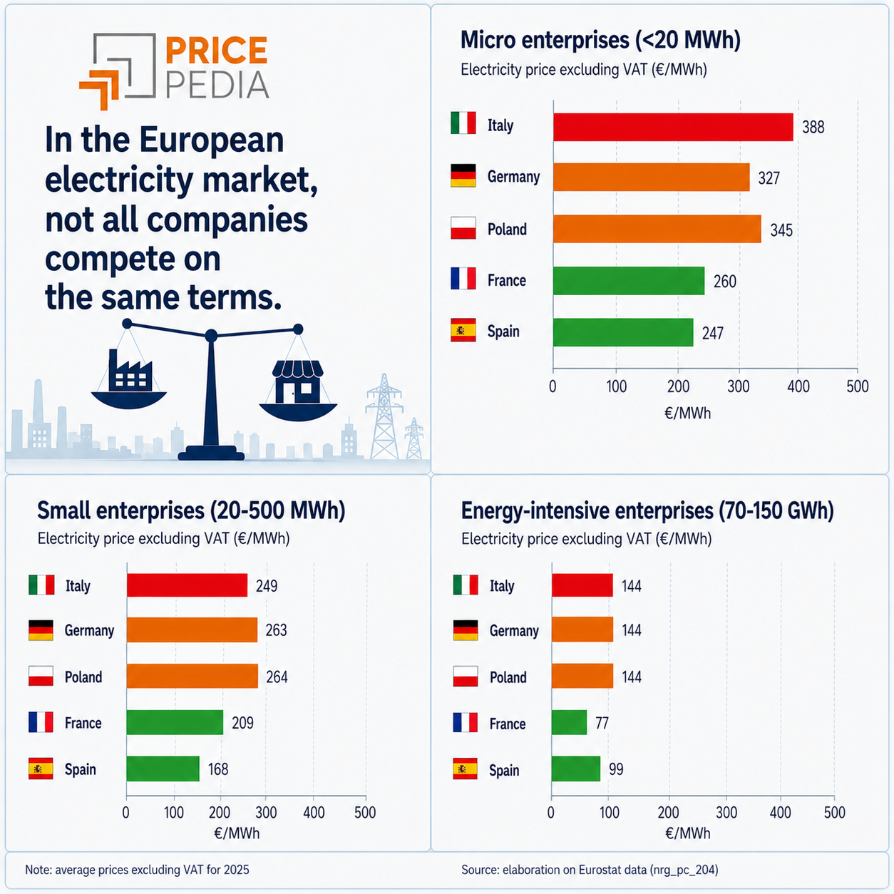
How Much Do European Companies Pay for Electricity?
Published by Luigi Bidoia. .
Electricity's National Single Price Electric Power Price DriversPrezzi diversi non solo tra mercati nazionali, ma anche in base ai livelli di consumo [ Read all ]
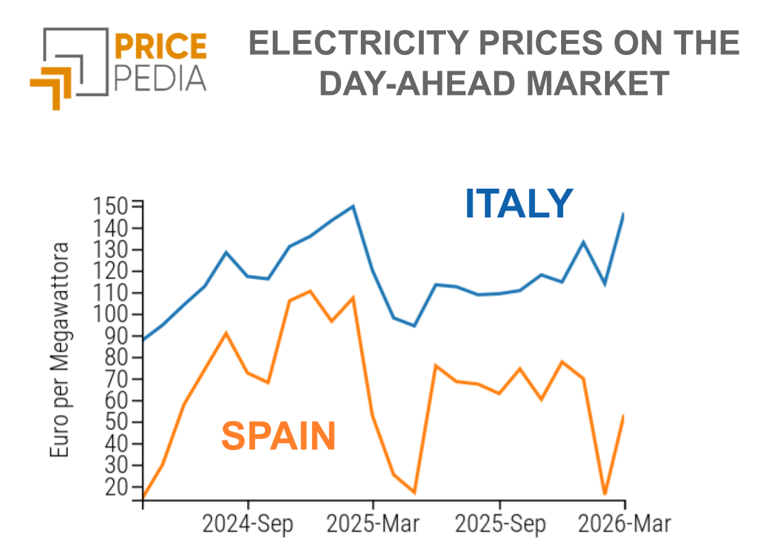
How Renewables Reduce the PUN’s Dependence on Gas Prices
Published by Luigi Bidoia. .
Electricity's National Single Price Electric Power Price DriversUna stima econometrica delle determinanti del PUN consente di misurare il contributo dei diversi fattori [ Read all ]

The impact of renewables on the PUN remains limited in the long run
Published by Luigi Bidoia. .
Electricity's National Single Price Electric Power Price DriversSono ancora poche le ore in cui le fonti rinnovabili determinano il prezzo [ Read all ]