The Microeconomic Approach to the Analysis of Commodity Markets: The Law of Supply and Demand
From theory to case analysis: how equilibrium varies based on elasticity
Published by Luigi Bidoia. .
economic analysis Analysis tools and methodologiesThe supply and demand model, also known as the partial equilibrium framework developed by Alfred Marshall, is one of the most fundamental and versatile tools in microeconomics. Although sometimes regarded as a simplification, this model proves particularly effective in analyzing commodity markets, where supply and demand interact in a structured way. In this article, we will explore how this model helps us understand the mechanisms that govern price formation and the quantities exchanged in competitive markets, characterized by the presence of numerous actors on both the supply and demand sides.
From Demand and Supply Equations to the Equilibrium Price
Economic theory has long examined demand and supply functions, highlighting the main factors that influence their behavior. In both cases, price is a central variable, but the relationship between price and quantity takes on fundamentally different characteristics in the case of demand compared to supply.
The Demand Function
In the case of demand[1],
a decrease in the price of a commodity tends to push a user firm to increase the quantity purchased.
A lower input cost can allow the firm to reduce the price of the finished product, stimulating final demand. To meet this increased demand, the firm is incentivized to expand production, and consequently, its purchases of the commodity used as input.
The opposite effect occurs when the price rises, reducing the incentive to produce and pushing firms to reduce demand for their inputs.
In short, there is an inverse relationship between price and quantity demanded: when the price changes, the quantity demanded tends to move in the opposite direction.
The Supply Function
The relationship between quantity and price is different in the supply function.
In a competitive market, the relationship between price and quantity supplied is direct: a price increase incentivizes producers to expand output, as it becomes economically more advantageous to bring larger quantities to market. Conversely, a price drop reduces the incentive to produce, leading suppliers to cut back on supply.
This positive relationship between price and quantity supplied is central to perfect competition models, where each firm takes the market price as given
and adjusts its level of production by comparing the market price with its own marginal cost[2].
The Equilibrium Price
Based on the behavior of producing and purchasing firms, as described respectively by the supply and demand functions,
the price of a commodity tends to vary until the quantity demanded and the quantity supplied coincide.
If, at a given price, the quantity demanded exceeds the quantity supplied, some purchasing firms will be willing to pay a higher price to obtain the desired quantity. This price increase will incentivize producers to expand their supply until the quantity produced matches the quantity requested: at that point, the market is in equilibrium.
Conversely, if the quantity demanded is lower than the quantity supplied, producers will be compelled to lower prices in order to sell all their output.
The price reduction will continue until the level of supply and demand coincide, determining a new market equilibrium.
Marshall's Equilibrium Model
To visually represent this adjustment process, Alfred Marshall, in his Principles of Economics published in 1890, plotted the demand and supply curves on a Cartesian plane, placing quantity on the horizontal axis and price on the vertical axis[3]. The result was the famous partial equilibrium model, which remains one of the fundamental tools for analyzing the functioning of competitive markets.

The supply and demand model, as represented by Marshall, offers a simple yet powerful tool for analyzing a wide range of real-world cases. To use it in a more refined way, however, it is necessary to introduce the concept of the price elasticity of demand and supply. When we talk about elasticity, we refer to the original demand and supply functions — that is, those expressing quantity as a function of price — and not to the inverse forms represented in Marshall’s diagram.
Price Elasticity of Demand and Supply
Elasticity measures how much the quantity demanded or supplied changes in response to a percentage change in price. A supply or demand is defined as inelastic when even large variations in price cause modest changes in quantity: graphically, the curves in the marshallian graph appear steep or almost vertical. In such cases, a market shock tends to produce large price fluctuations and only limited changes in traded quantities. Conversely, when demand or supply is highly elastic — meaning a small change in price leads to large changes in quantity — the supply and demand curves in the marshallian graph are almost flat, and market shocks mainly translate into quantity adjustments, with smaller effects on prices.
Introducing the concept of elasticity is useful for analyzing how market equilibrium adjusts in the short run versus the long run in response to demand or supply shocks.
In the short run, the price elasticity of demand is generally low, because user firms have limited options for substituting one commodity with another: production processes are already in place, existing contracts constrain choices, and uncertainty discourages change. In the long run, however, the potential for input substitution increases thanks to investments in new technologies, changes in production cycles, or more flexible sourcing strategies — making demand more elastic.
A similar logic applies to supply. In the short run, production is constrained by fixed factors — such as installed capacity, labor contracts, or raw material availability — which make supply less responsive to price changes. But in the long run, all production factors become variable: firms can expand capacity, access new inputs, and reorganize production. This makes supply much more elastic and better able to adapt to new market conditions.
Market Adjustment in the Short and Long Run
The following two figures represent the market framework in the short run and the long run. They illustrate how the system reaches a new equilibrium following a demand-side shock, indicated as a rightward shift of the demand curve.
The diagrams clearly show that in the short run — characterized by low elasticity and nearly vertical curves — the adjustment occurs mainly through a sharp increase in price, while the change in traded quantities is relatively limited. The opposite happens in the long run: when demand and supply become more elastic (flatter curves), the adjustment focuses on quantities, with more moderate price variations.

This analysis provides a solid theoretical foundation for interpreting the behavior observed in commodity markets, where shocks — such as geopolitical events, logistics crises, unexpected surges in demand, or force majeure events on the supply side — generate strong price volatility in the short term. However, over time, behavioral adjustments and investment responses lead prices to gradually absorb the initial shock, converging toward long-run levels.
This characteristic of commodity markets makes it essential to study the mechanisms that determine long-term prices, since despite short-term turbulence, the market tends to stabilize around these underlying values.
Summary
The neoclassical price determination model, developed by Marshall, offers an effective representation of competitive mechanisms in standardized commodity markets. It can be easily used to provide a theoretical foundation for an empirical pattern common to most of these markets: the ongoing sequence of cyclical phases in price dynamics. The price level of a commodity can, in fact, be broken down into two components:
- a long-run component, determined by structural factors such as long-term demand and supply, production technology, input prices, and consequently, production costs;
- a short-run component, much more volatile, driven by temporary factors such as inventory policies of user firms, production disruptions, logistical delays, or speculative actions in distribution. It is precisely this component, which tends to fluctuate around zero, that generates the cyclical phases observed in prices.
The ability to decompose the commodity price into these two components is essential for building reliable forecasting scenarios and for correctly interpreting market dynamics.
[1] In microeconomics, the demand for a production input is commonly analyzed within the framework of a profit-maximizing firm, by studying the behavior of demand for a variable factor. The formal characteristics of the resulting demand curve are similar to those of a consumer’s demand curve for a consumption good under utility maximization, although the two are derived from different theoretical frameworks and respond to distinct economic determinants.
[2] A firm is incentivized to increase production as long as the revenue from the additional unit (given by the price) exceeds the cost required to produce it (marginal cost).
[3] Although the demand and supply “curves” commonly shown on Cartesian axes are often referred to as standard functions, it should be noted that Marshall used the inverse functions: price is expressed as a function of quantity, not the other way around. Formally, Marshall's curves are represented as P = D⁻¹(Q) and P = S⁻¹(Q), rather than Q = D(P) or Q = S(P). This graphical choice highlights how price adjusts in response to imbalances between demand and supply.
You may be interested in:
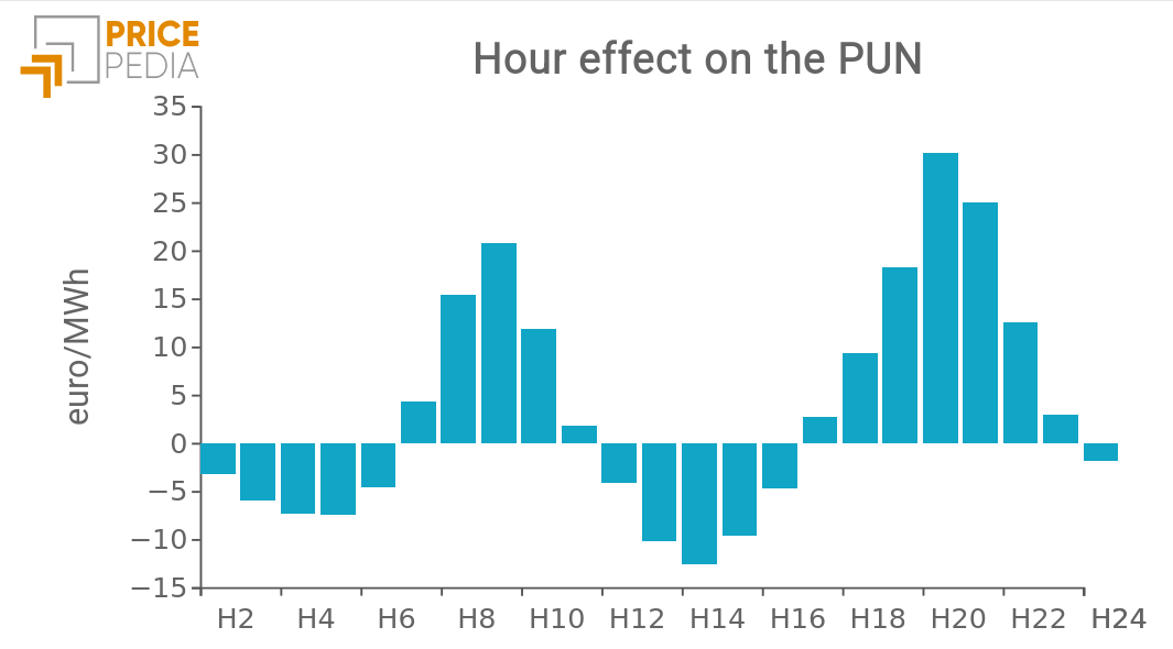
Hourly PUN price: is there a specific “hour” effect?
Published by Emanuele Morelli. .
Electricity's National Single Price Electric Power economic analysis Machine learning and EconometricsAn econometric analysis reveals the existence of a temporal pattern in electricity prices. [ Read all ]
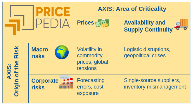
Macro commodity risks and corporate procurement risks
Published by Cristina Luca. .
Procurement economic analysis Procurement Risk ManagementHow procurement management is evolving in an uncertain world [ Read all ]

Physical Prices, Financial Prices, and Risk Transmission: An Analysis of Correlations
Published by Cristina Luca. .
economic analysis Analysis tools and methodologiesAnalisi quantitativa delle correlazioni tra prezzi fisici e finanziari [ Read all ]