Commodities and Volatility: How to Measure and Manage Risk in Global Markets
Published by Cristina Luca. .
economic analysis Analysis tools and methodologiesCommodity Risk and Price Volatility
Commodity risk can be defined as the set of threats arising from both systemic market factors and company-specific elements that affect the supply, cost, and availability of raw materials. These factors have macroeconomic, strategic, or environmental origins.
For this reason, it is essential to measure the degree of risk exposure that each operator — particularly those involved in procurement — faces. Among the various components of commodity risk, price volatility plays a central role, as it reflects the uncertainty that characterizes markets and directly impacts procurement strategies.
Volatility represents the degree of price variability over time. Put simply, high volatility signals strong and unpredictable price swings, while low volatility indicates greater price stability and predictability.
It is influenced by a wide range of factors, mostly macroeconomic: geopolitical events (wars, sanctions), fluctuations in exchange rates, inflation, and interest rates, speculative activity in financial markets, as well as environmental or climate-related events. In addition, demand or supply shocks may trigger sudden and significant changes in price levels.
Volatility and the Role of Market Players: Comparing Speculators and Buyers
Volatility does not have a single, fixed meaning: its interpretation depends on the profile of the operator.
For a speculator, it can represent an opportunity. These actors are not concerned with the direction of prices—whether they rise or fall—but rather with their ability to anticipate price movements in order to profit from the fluctuations. From this perspective, volatility is neutral: it is the condition that makes profit generation possible.
For a buyer, on the other hand, volatility represents a source of uncertainty and a potential operational risk. Price increases can lead to higher input costs, squeeze profit margins, and undermine commercial strategies based on fixed prices or long-term contracts.
Even a price decrease, although it may initially seem positive (cheaper inputs), must be assessed cautiously: it can lead suppliers to delay deliveries, renegotiate contract terms, or signal a contraction in demand due to an economic slowdown—which in turn constitutes an additional risk factor.
What makes risk management even more complex is that in commodity markets, physical prices—that is, the prices actually paid for purchasing and delivering raw materials—are strongly influenced by financial prices, which are determined on global markets through derivatives such as futures contracts.
A telling example is copper: the financial price not only affects the value of the raw material itself but also that of the first industrial transformations, such as copper wires and tubes. Consequently, financial price volatility tends to transmit to physical prices as well, generating uncertainty and increasing the level of risk for those involved in procurement.
Financial Price Volatility of Commodities
Generally, the volatility of a financial asset (for example, the quotation of a futures contract underlying a commodity price) is calculated as the coefficient of variation of prices, i.e., the ratio between the standard deviation and the average price over a given period. However, since the behavior of a time series can be described both by its internal variability and its overall net change, a synthetic measure integrating both components has been adopted. This allows a more comprehensive assessment of the dynamic intensity of the process.
Nonetheless, the choice of the time horizon over which to calculate these measures remains central. For a trader operating with intraday strategies, the reference horizon can be extremely short, down to a single day. Conversely, for an economic operator interested in assessing uncertainty over longer horizons, the interval can extend over several months, up to an entire year.
To accommodate these different informational needs, we have calculated three distinct volatility measures, based on both the coefficient of variation and the absolute percentage change, with weekly, monthly, and annual frequencies, comparing two historical periods: the pre-pandemic five-year period (2015–2020) and the subsequent one (2020–2025). The goal is to verify whether the extraordinary events of recent years have structurally altered the volatility profile of the markets.
The following table shows financial price volatility[1] calculated by macro-categories of commodities, comparing the two periods analyzed and highlighting the difference between them.
Financial Price Volatility by Commodity Macro-Categories
| PricePedia Product Families | Periods | Difference Between Periods | |
|---|---|---|---|
| Jan 2015–Dec 2019 | Jan 2020–Dec 2024 | ||
| Energy | 10.14 | 19.36 | 9.22 |
| Wood and Paper | 5.95 | 9.27 | 3.31 |
| Ferrous Metals | 7.94 | 9.20 | 1.25 |
| Food | 5.29 | 8.21 | 2.92 |
| Organic Chemicals | 6.13 | 7.86 | 1.73 |
| Textile Fibers | 5.12 | 7.79 | 2.67 |
| Non-Ferrous Metals | 6.21 | 7.50 | 1.29 |
| Plastics and Elastomers | 6.32 | 7.49 | 1.17 |
| Precious Metals | 5.51 | 7.01 | 1.50 |
The analysis of financial price volatility by major commodity categories shows a generalized increase in the post-pandemic period (2020–2024) compared to the previous five years (2015–2019).
Among the various categories, Energy commodities recorded the most significant increase, with an average rise of over 9 percentage points, followed by Wood and Paper, Ferrous metals, and Food. This increase reflects the instability caused by the pandemic, the energy crisis, and geopolitical tensions, which have disrupted the regularity of global value chains.
In contrast, the Precious metals, Plastics and Elastomers, and Non-Ferrous metals categories rank among the least volatile, although they still registered an increase in the most recent period.
Going into more detail, the following tables show the volatility and changes between the two periods considered, referring to some financial prices of individual commodities.
Financial Prices of Commodities with the Highest Volatility
| PricePedia Product Families | Individual Product | Periods | Difference between the two periods | |
|---|---|---|---|---|
| Jan 2015 – Dec 2019 | Jan 2020 – Dec 2024 | |||
| Energy | Natural Gas TTF (Netherlands) (ICE), price/MWh | 10.61 | 39.04 | 28.43 |
| Energy | Natural Gas NBP (UK) (ICE), price/Therm | 11.19 | 38.08 | 26.89 |
| Energy | Liquefied Natural Gas JKM (Asia) (CME), price/MMBtu | 12.46 | 33.04 | 20.58 |
| Energy | WTI (CME), price/barrel | 9.79 | 22.68 | 12.89 |
| Energy | Thermal Coal Australia (ICE) | 8.39 | 21.22 | 12.83 |
| Wood and Paper | Recycled Paper OCC (NOREXECO) | 6.55 | 19.53 | 12.98 |
| Energy | Natural Gas Henry Hub (USA) (NYMEX), price/MMBtu | 9.61 | 18.03 | 8.42 |
| Wood and Paper | US Softwood Lumber (CME), price/Thousand Board Feet | 8.88 | 16.07 | 7.19 |
| Ferrous | Hot Rolled Coils USA (CME), price/Short Ton | 8.46 | 15.91 | 7.45 |
| Energy | Liquefied Propane (CME), price/Gallon | 12.71 | 14.09 | 1.38 |
At the individual product level, the highest volatility is clearly concentrated within the Energy family. At the top of the ranking are Natural Gas TTF, the British NBP Gas, and Liquefied Natural Gas JKM, all with volatility increases exceeding 20 percentage points. The WTI Crude Oil also showed an exceptional dynamic, culminating in the historic episode of April 2020 when the price temporarily dropped below zero.
Financial Prices of Commodities with the Lowest Volatility
| PricePedia Product Families | Individual Product | Periods | Difference between the two periods | |
|---|---|---|---|---|
| Jan 2015 – Dec 2019 | Jan 2020 – Dec 2024 | |||
| Non-Ferrous | Lead (SHFE) | 5.25 | 3.38 | -1.87 |
| Food | Raw Sugar 16 (ICE), price/Pound | 2.69 | 3.99 | 1.30 |
| Precious Metals | Gold (CME), price/Troy Ounce | 3.24 | 4.52 | 1.28 |
| Plastics and Elastomers | Polypropylene China (DCE) | 6.67 | 4.69 | -1.98 |
| Plastics and Elastomers | LLDPE China (DCE) | 5.11 | 4.87 | -0.24 |
| Food | Raw Rice (CME), price/Short Hundredweight | 5.72 | 5.56 | -0.16 |
| Wood and Paper | NBSK Pulp Europe (NOREXECO) | 3.82 | 5.63 | 1.81 |
| Non-Ferrous | Aluminum (SHFE) | 4.16 | 5.91 | 1.75 |
| Non-Ferrous | Copper (SHFE) | 5.31 | 6.10 | 0.79 |
| Non-Ferrous | Zinc (SHFE) | 6.72 | 6.19 | -0.52 |
Among the less volatile commodities are metals such as Lead, Aluminum, Copper, and Zinc, food products such as Rice and Sugar, and plastics such as Polypropylene and LLDPE (both traded in China), which have maintained contained volatility over time.
Also noteworthy is Gold, which, despite registering a slight increase, confirms its role as a safe haven during turbulent times, with one of the lowest volatilities among all the commodities analyzed.
Particularly interesting is the case of the Food sector, which overall has registered an average increase in volatility but is less homogeneous compared to other families. The presence of very stable products within it, such as Rice and Sugar, balances the high instability of raw materials like Cocoa and Coffee, whose volatility has been among the highest, although they do not appear among the top ten most volatile products overall.
Conclusions
Having calculated the financial price volatility indicator of commodities, one can proceed towards a broader analysis. As mentioned earlier, financial price volatility tends to transmit or influence that of physical prices.
Therefore, starting from this initial indicator, it is possible to develop a further indicator aimed at measuring and interpreting the volatility of physical commodity prices,
thus providing a more complete framework of physical price risks, related to the actual purchases of processors.
[1] A value of 10 means, for example, that the price has experienced a coefficient of variation and an absolute average weekly, monthly, annual change of, on average, 10%.
You may be interested in:
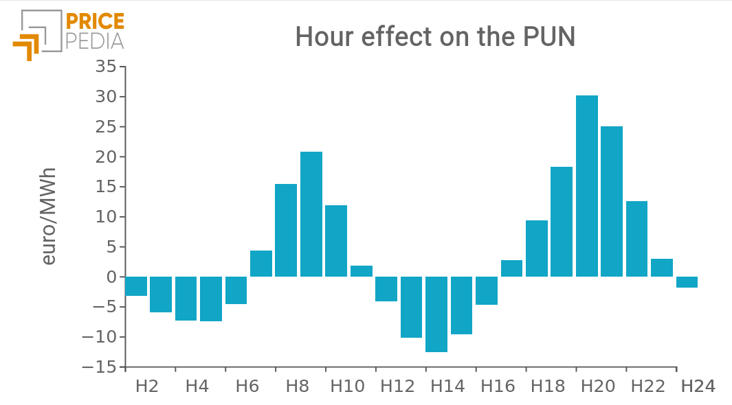
Hourly PUN price: is there a specific “hour” effect?
Published by Emanuele Morelli. .
Electricity's National Single Price Electric Power economic analysis Machine learning and EconometricsAn econometric analysis reveals the existence of a temporal pattern in electricity prices. [ Read all ]
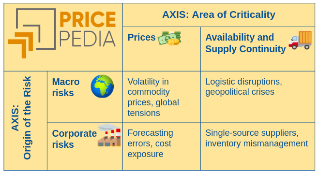
Macro commodity risks and corporate procurement risks
Published by Cristina Luca. .
Procurement economic analysis Procurement Risk ManagementHow procurement management is evolving in an uncertain world [ Read all ]
Physical Prices, Financial Prices, and Risk Transmission: An Analysis of Correlations
Published by Cristina Luca. .
economic analysis Analysis tools and methodologiesAnalisi quantitativa delle correlazioni tra prezzi fisici e finanziari [ Read all ]